Graphs
A Graph is a non-linear data structure that consists of vertices (nodes) and edges.
A vertex, also called a node, is a point or an object in the Graph, and an edge is used to connect two vertices with each other.
Graphs are non-linear because the data structure allows us to have different paths to get from one vertex to another, unlike with linear data structures like Arrays or Linked Lists.
Graphs are used to represent and solve problems where the data consists of objects and relationships between them
Examples:
Social Networks: Each person is a vertex, and relationships (like friendships) are the edges. Algorithms can suggest potential friends.
Maps and Navigation: Locations, like a town or bus stops, are stored as vertices, and roads are stored as edges. Algorithms can find the shortest route between two locations when stored as a Graph.
Internet: Can be represented as a Graph, with web pages as vertices and hyperlinks as edges.
Biology: Graphs can model systems like neural networks or the spread of diseases.
வரைபடம் (கிராஃப்)
ஒரு வரைபடம் என்பது உச்சிகள் (முனைகள்) மற்றும் விளிம்புகளைக் கொண்ட ஒரு நேரியல் அல்லாத தரவுக் கட்டமைப்பாகும்.
முனை என்றும் அழைக்கப்படும் ஒரு உச்சி, வரைபடத்தில் உள்ள ஒரு புள்ளி அல்லது ஒரு பொருளாகும், மேலும் இரண்டு உச்சிகளை ஒன்றோடொன்று இணைக்க ஒரு விளிம்பு பயன்படுத்தப்படுகிறது.
அணிகள் அல்லது இணைக்கப்பட்ட பட்டியல்கள் போன்ற நேரியல் தரவுக் கட்டமைப்புகளைப் போலல்லாமல், ஒரு உச்சியிலிருந்து மற்றொரு உச்சிக்குச் செல்ல வெவ்வேறு பாதைகளை இந்தத் தரவுக் கட்டமைப்பு அனுமதிப்பதால், வரைபடங்கள் நேரியல் அல்லாதவை ஆகும்.
தரவு என்பது பொருட்களையும் அவற்றுக்கிடையேயான உறவுகளையும் கொண்டிருக்கும் சிக்கல்களைப் பிரதிநிதித்துவப்படுத்தவும் தீர்க்கவும் வரைபடங்கள் பயன்படுத்தப்படுகின்றன.
உதாரணங்கள்:
சமூக வலைப்பின்னல்கள்: ஒவ்வொரு நபரும் ஒரு உச்சியாகவும், உறவுகள் (நட்புகள் போன்றவை) விளிம்புகளாகவும் உள்ளன. வழிமுறைகள் சாத்தியமான நண்பர்களைப் பரிந்துரைக்க முடியும்.
வரைபடங்கள் மற்றும் வழிசெலுத்தல்: ஒரு நகரம் அல்லது பேருந்து நிறுத்தங்கள் போன்ற இடங்கள் உச்சிகளாகவும், சாலைகள் விளிம்புகளாகவும் சேமிக்கப்படுகின்றன. ஒரு வரைபடமாகச் சேமிக்கப்படும்போது, இரண்டு இடங்களுக்கு இடையே உள்ள குறுகிய வழியை வழிமுறைகள் கண்டறிய முடியும்.
இணையம்: வலைப்பக்கங்களை உச்சிகளாகவும், ஹைப்பர்லிங்குகளை விளிம்புகளாகவும் கொண்டு இணையத்தை ஒரு வரைபடமாகப் பிரதிநிதித்துவப்படுத்தலாம்.
உயிரியல்: நரம்பு மண்டலங்கள் அல்லது நோய்கள் பரவுதல் போன்ற அமைப்புகளை வரைபடங்கள் மூலம் மாதிரியாக்கலாம்.
Graph Properties
A weighted Graph is a Graph where the edges have values. The weight value of an edge can represent things like distance, capacity, time, or probability.
A connected Graph is when all the vertices are connected through edges somehow. A Graph that is not connected, is a Graph with isolated (disjoint) subgraphs, or single isolated vertices.
A directed Graph, also known as a digraph, is when the edges between the vertex pairs have a direction. The direction of an edge can represent things like hierarchy or flow.
A cyclic Graph is defined differently depending on whether it is directed or not:
A directed cyclic Graph is when you can follow a path along the directed edges that goes in circles. Removing the directed edge from Apple to Coffee in the animation above makes the directed Graph not cyclic anymore.
An undirected cyclic Graph is when you can come back to the same vertex you started at without using the same edge more than once. The undirected Graph above is cyclic because we can start and end up in vertes Coffee without using the same edge twice.
A loop, also called a self-loop, is an edge that begins and ends on the same vertex. A loop is a cycle that only consists of one edge. By adding the loop on vertex Apple in the animation above, the Graph becomes cyclic.
வரைபடப் பண்புகள்
எடைகொண்ட வரைபடம் என்பது விளிம்புகள் மதிப்புகளைக் கொண்ட ஒரு வரைபடமாகும். ஒரு விளிம்பின் எடை மதிப்பு தூரம், கொள்ளளவு, நேரம் அல்லது நிகழ்தகவு போன்ற விஷயங்களைக் குறிக்கலாம்.
இணைக்கப்பட்ட வரைபடம் என்பது அனைத்து முனைகளும் ஏதேனும் ஒரு வகையில் விளிம்புகள் வழியாக இணைக்கப்பட்டிருக்கும் நிலையாகும். இணைக்கப்படாத வரைபடம் என்பது தனிமைப்படுத்தப்பட்ட (தொடர்பற்ற) துணை வரைபடங்கள் அல்லது தனித்தனி முனைகளைக் கொண்ட ஒரு வரைபடமாகும்.
திசையிடப்பட்ட வரைபடம், இது டைகிராஃப் என்றும் அழைக்கப்படுகிறது, என்பது முனை ஜோடிகளுக்கு இடையிலான விளிம்புகள் ஒரு திசையைக் கொண்டிருக்கும் நிலையாகும். ஒரு விளிம்பின் திசையானது படிநிலை அல்லது ஓட்டம் போன்ற விஷயங்களைக் குறிக்கலாம்.
ஒரு சுழற்சி வரைபடம் என்பது அது திசையிடப்பட்டதா இல்லையா என்பதைப் பொறுத்து வித்தியாசமாக வரையறுக்கப்படுகிறது:
ஒரு திசையிடப்பட்ட சுழற்சி வரைபடம் என்பது, திசையிடப்பட்ட விளிம்புகள் வழியாக வட்டமாகச் செல்லும் ஒரு பாதையைப் பின்பற்ற முடிந்தால் ஆகும். மேலே உள்ள அசைவூட்டத்தில் ஆப்பிளிலிருந்து காபிக்குச் செல்லும் திசையிடப்பட்ட விளிம்பை நீக்குவது, அந்த திசையிடப்பட்ட வரைபடத்தை இனி சுழற்சி அற்றதாக ஆக்குகிறது.
ஒரு திசையிடப்படாத சுழற்சி வரைபடம் என்பது, ஒரே விளிம்பை ஒன்றுக்கு மேற்பட்ட முறை பயன்படுத்தாமல், நீங்கள் தொடங்கிய அதே முனைக்குத் திரும்ப முடிந்தால் ஆகும். மேலே உள்ள திசையிடப்படாத வரைபடம் சுழற்சி கொண்டது, ஏனெனில் நாம் ஒரே விளிம்பை இருமுறை பயன்படுத்தாமல் காபி முனையில் தொடங்கி அங்கேயே முடிக்க முடியும்.
ஒரு கண்ணி, இது சுய-கண்ணி என்றும் அழைக்கப்படுகிறது, என்பது ஒரே முனையில் தொடங்கி முடிவடையும் ஒரு விளிம்பாகும். ஒரு கண்ணி என்பது ஒரே ஒரு விளிம்பைக் கொண்ட ஒரு சுழற்சியாகும். மேலே உள்ள அசைவூட்டத்தில் ஆப்பிள் முனையில் கண்ணியைச் சேர்ப்பதன் மூலம், அந்த வரைபடம் சுழற்சி கொண்டதாகிறது.
Graph Representations
A Graph representation tells us how a Graph is stored in memory.
Different Graph representations can:
- take up more or less space.
- be faster or slower to search or manipulate.
- be better suited depending on what type of Graph we have (weighted, directed, etc.), and what we want to do with the Graph.
- be easier to understand and implement than others.
Graph representations store information about which vertices are adjacent, and how the edges between the vertices are. Graph representations are slightly different if the edges are directed or weighted.
Two vertices are adjacent, or neighbors, if there is an edge between them.
வரைபடப் பிரதிநிதித்துவங்கள்
ஒரு வரைபடம் நினைவகத்தில் எவ்வாறு சேமிக்கப்படுகிறது என்பதை வரைபடப் பிரதிநிதித்துவம் நமக்குச் சொல்கிறது.
வெவ்வேறு வரைபடப் பிரதிநிதித்துவங்கள்:
- அதிகமாகவோ அல்லது குறைவாகவோ இடத்தை எடுத்துக் கொள்ளலாம்.
- தேட அல்லது கையாள வேகமாகவோ அல்லது மெதுவாகவோ இருக்கலாம்.
- நம்மிடம் உள்ள வரைபட வகை (எடையிடப்பட்டது, இயக்கப்பட்டது போன்றவை) மற்றும் வரைபடத்துடன் நாம் என்ன செய்ய விரும்புகிறோம் என்பதைப் பொறுத்து சிறப்பாகப் பொருந்தலாம்.
- மற்றவற்றை விட புரிந்துகொள்வதற்கும் செயல்படுத்துவதற்கும் எளிதாக இருக்கும்.
வரைபடப் பிரதிநிதித்துவங்கள் எந்த முனைகள் அருகில் உள்ளன, மற்றும் முனைகளுக்கு இடையிலான விளிம்புகள் எவ்வாறு உள்ளன என்பது பற்றிய தகவல்களைச் சேமிக்கின்றன. விளிம்புகள் இயக்கப்பட்டாலோ அல்லது எடையிடப்பட்டாலோ வரைபடப் பிரதிநிதித்துவங்கள் சற்று வித்தியாசமாக இருக்கும்.
இரண்டு முனைகள் அருகில் உள்ளன, அல்லது அவற்றுக்கிடையே ஒரு விளிம்பு இருந்தால், அண்டை வீட்டாராக இருக்கும்.
Adjacency Matrix Graph Representation
Adjacency Matrix is the Graph representation (structure) we will use for this tutorial.
The Adjacency Matrix is a 2D array (matrix) where each cell on index (i,j) stores information about the edge from vertex i to vertex j.
Below is a Graph with the Adjacency Matrix representation next to it.
அண்மை அணி வரைபடப் பிரதிநிதித்துவம்
இந்த டுடோரியலுக்காக நாம் பயன்படுத்தப் போகும் வரைபடப் பிரதிநிதித்துவம் (அமைப்பு) அண்மை அணி ஆகும்.
அண்மை அணி என்பது ஒரு 2D அணி (மேட்ரிக்ஸ்) ஆகும், இதில் (i,j) குறியீட்டில் உள்ள ஒவ்வொரு கலமும், i முனையிலிருந்து j முனைக்குச் செல்லும் விளிம்பைப் பற்றிய தகவல்களைச் சேமிக்கிறது.
கீழே ஒரு வரைபடமும், அதற்கு அருகில் அதன் அண்மை அணிப் பிரதிநிதித்துவமும் கொடுக்கப்பட்டுள்ளது.
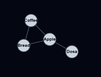
| Apple | Bread | Coffee | Dosa | |
| Apple | 1 | 1 | 1 | |
| Bread | 1 | 1 | ||
| Coffee | 1 | 1 | ||
| Dosa | 1 |
An undirected Graph and the adjacency matrix
The adjacency matrix above represents an undirected Graph, so the values ‘1’ only tells us where the edges are. Also, the values in the adjacency matrix is symmetrical because the edges go both ways (undirected Graph).
திசையற்ற வரைபடம் மற்றும் அண்மை அணி
மேலே உள்ள அண்மை அணியானது ஒரு திசையற்ற வரைபடத்தைக் குறிக்கிறது, எனவே ‘1’ என்ற மதிப்புகள் விளிம்புகள் எங்கு அமைந்துள்ளன என்பதை மட்டுமே நமக்குத் தெரிவிக்கின்றன. மேலும், இது ஒரு திசையற்ற வரைபடம் என்பதால், விளிம்புகள் இரு வழிகளிலும் செல்வதால், அண்மை அணியில் உள்ள மதிப்புகள் சமச்சீராக உள்ளன.
Below is a directed and weighted Graph with the Adjacency Matrix representation next to it.
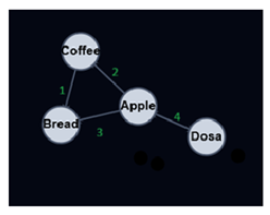
| Apple | Bread | Coffee | Dosa | |
| Apple | 3 | 2 | ||
| Bread | ||||
| Coffee | 1 | |||
| Dosa | 4 |
A directed and weighted Graph,and its adjacency matrix.
In the adjacency matrix above, the value 3 on index (0,1) tells us there is an edge from vertex Apple to vertex Bread, and the weight for that edge is 3.
As you can see, the weights are placed directly into the adjacency matrix for the correct edge, and for a directed Graph, the adjacency matrix does not have to be symmetric.
Adjacency List Graph Representation
In case we have a ‘sparse’ Graph with many vertices, we can save space by using an Adjacency List compared to using an Adjacency Matrix, because an Adjacency Matrix would reserve a lot of memory on empty Array elements for edges that don’t exist.
A ‘sparse’ Graph is a Graph where each vertex only has edges to a small portion of the other vertices in the Graph.
An Adjacency List has an array that contains all the vertices in the Graph, and each vertex has a Linked List (or Array) with the vertex’s edges.
அண்மைப் பட்டியல் வரைபடப் பிரதிநிதித்துவம்
பல முனைகளைக் கொண்ட ஒரு ‘அடர்த்தி குறைந்த’ வரைபடம் நம்மிடம் இருக்கும் பட்சத்தில், அண்மை அணிக்குப் பதிலாக அண்மைப் பட்டியலைப் பயன்படுத்துவதன் மூலம் நாம் நினைவக இடத்தை மிச்சப்படுத்தலாம். ஏனெனில், அண்மை அணியானது இல்லாத விளிம்புகளுக்கான காலி அணி உறுப்புகளுக்கு அதிக நினைவகத்தை ஒதுக்கும்.
ஒரு ‘அடர்த்தி குறைந்த’ வரைபடம் என்பது, அதில் உள்ள ஒவ்வொரு முனையும், வரைபடத்தில் உள்ள மற்ற முனைகளில் ஒரு சிறிய பகுதிக்கு மட்டுமே விளிம்புகளைக் கொண்டிருக்கும் ஒரு வரைபடமாகும்.
ஒரு அண்மைப் பட்டியலில், வரைபடத்தில் உள்ள அனைத்து முனைகளையும் கொண்ட ஒரு அணி இருக்கும், மேலும் ஒவ்வொரு முனையும் அந்த முனையின் விளிம்புகளைக் கொண்ட ஒரு இணைக்கப்பட்ட பட்டியலைக் (அல்லது அணியைக்) கொண்டிருக்கும்.
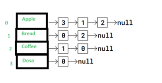
In the adjacency list above, the vertices Apple to Dosa are placed in an Array, and each vertex in the array has its index written right next to it.
Each vertex in the Array has a pointer to a Linked List that represents that vertex’s edges. More specifically, the Linked List contains the indexes to the adjacent (neighbor) vertices.
So for example, vertex Apple has a link to a Linked List with values 3, 1, and 2. These values are the indexes to Apple’s adjacent vertices Dosa, Bread, and Coffee.
மேலே உள்ள அண்மைப் பட்டியலில், ஆப்பிள் முதல் தோசை வரையிலான முனைகள் ஒரு வரிசையில் (அரேயில்) வைக்கப்பட்டுள்ளன, மேலும் அந்த வரிசையில் உள்ள ஒவ்வொரு முனைக்கும் அதன் குறியீட்டு எண் அதற்கு நேராகவே எழுதப்பட்டுள்ளது.
அந்த வரிசையில் உள்ள ஒவ்வொரு முனைக்கும், அந்த முனையின் விளிம்புகளைக் குறிக்கும் ஒரு இணைக்கப்பட்ட பட்டியலுக்கான சுட்டிக்காட்டி (pointer) உள்ளது. இன்னும் குறிப்பாகச் சொன்னால், அந்த இணைக்கப்பட்ட பட்டியலில், அருகிலுள்ள (அண்டை) முனைகளின் குறியீட்டு எண்கள் உள்ளன.
உதாரணமாக, ஆப்பிள் என்ற முனைக்கு 3, 1, மற்றும் 2 ஆகிய மதிப்புகளைக் கொண்ட ஒரு இணைக்கப்பட்ட பட்டியலுக்கான இணைப்பு உள்ளது. இந்த மதிப்புகள், ஆப்பிளின் அண்டை முனைகளான தோசை, பிரெட் மற்றும் காபி ஆகியவற்றின் குறியீட்டு எண்களாகும்.
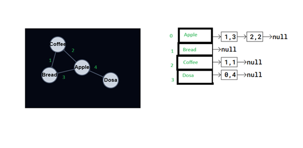
An Adjacency List can also represent a directed and weighted Graph, like this:
A directed and weighted Graph and its adjacency list.
In the Adjacency List above, vertices are stored in an Array. Each vertex has a pointer to a Linked List with edges stored as i,w, where i is the index of the vertex the edge goes to, and w is the weight of that edge.
Node ‘Dosa’ for example, has a pointer to a Linked List with an edge to vertex ‘Apple’. The values 0,4 means that vertex ‘Dosa’ has an edge to vertex on index 0 (vertex ‘Apple’), and the weight of that edge is 4.
ஒரு திசை மற்றும் எடை கொண்ட வரைபடத்தையும் (directed and weighted Graph) ஒரு அண்மைப் பட்டியல் மூலம் இவ்வாறு குறிப்பிடலாம்:
ஒரு திசை மற்றும் எடை கொண்ட வரைபடம் மற்றும் அதன் அண்மைப் பட்டியல்.
மேலே உள்ள அண்மைப் பட்டியலில், முனைகள் ஒரு வரிசையில் சேமிக்கப்பட்டுள்ளன. ஒவ்வொரு முனைக்கும் ஒரு இணைக்கப்பட்ட பட்டியலுக்கான சுட்டிக்காட்டி உள்ளது. அந்தப் பட்டியலில் விளிம்புகள் i,w என சேமிக்கப்பட்டுள்ளன, இங்கு i என்பது அந்த விளிம்பு செல்லும் முனையின் குறியீடு, மற்றும் w என்பது அந்த விளிம்பின் எடை ஆகும்.
உதாரணமாக, ‘Dosa’ என்ற முனை, ‘Apple’ என்ற முனைக்குச் செல்லும் ஒரு விளிம்பைக் கொண்ட இணைக்கப்பட்ட பட்டியலுக்கான ஒரு சுட்டிக்காட்டியைக் கொண்டுள்ளது. 0,4 என்ற மதிப்புகள், ‘Dosa’ என்ற முனையிலிருந்து குறியீடு 0-இல் உள்ள முனைக்கு (‘Apple’ என்ற முனைக்கு) ஒரு விளிம்பு உள்ளது என்பதையும், அந்த விளிம்பின் எடை 4 என்பதையும் குறிக்கிறது.
Graphs Implementation
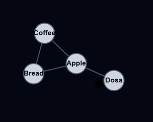
To implement a Graph we will use an Adjacency Matrix, like the one below.
ஒரு வரைபடத்தை (Graph) செயல்படுத்த, கீழே உள்ளதைப் போன்ற ஒரு அண்மை அணி (Adjacency Matrix) பயன்படுத்தப்படும்.

| Apple | Bread | Coffee | Dosa | |
| Apple | 1 | 1 | 1 | |
| Bread | 1 | 1 | ||
| Coffee | 1 | 1 | ||
| Dosa | 1 |
To store data for each vertex, in this case the letters Apple, Bread, Coffee, and Dosa, the data is put in a separate array that matches the indexes in the adjacency matrix, like this:
For an undirected and not weighted Graph, like in the image above, an edge between vertices i and j is stored with value 1. It is stored as 1 on both places (j,i) and (i,j) because the edge goes in both directions. As you can see, the matrix becomes diagonally symmetric for such undirected Graphs.
Let’s look at something more specific. In the adjacency matrix above, vertex ‘Apple’ is on index 0, and vertex ‘Dosa’ is on index 3, so we get the edge between ‘Apple’ and ‘Dosa’ stored as value 1 in position (0,3) and (3,0), because the edge goes in both directions.
ஒவ்வொரு முனைப்புள்ளிக்குமான தரவைச் சேமிக்க, இந்தச் சந்தர்ப்பத்தில் ஆப்பிள், பிரெட், காபி மற்றும் தோசை ஆகிய வார்த்தைகளை, அருகாமை அணிவரிசையில் உள்ள குறியீடுகளுடன் பொருந்தக்கூடிய ஒரு தனி வரிசையில் தரவு வைக்கப்படுகிறது, இது பின்வருமாறு:
மேலே உள்ள படத்தில் உள்ளதைப் போன்ற திசையற்ற மற்றும் எடையற்ற வரைபடத்திற்கு, i மற்றும் j ஆகிய முனைப்புள்ளிகளுக்கு இடையிலான ஒரு விளிம்பு 1 என்ற மதிப்புடன் சேமிக்கப்படுகிறது. அந்த விளிம்பு இரு திசைகளிலும் செல்வதால், அது (j,i) மற்றும் (i,j) ஆகிய இரண்டு இடங்களிலும் 1 ஆகச் சேமிக்கப்படுகிறது. நீங்கள் பார்க்கிறபடி, இத்தகைய திசையற்ற வரைபடங்களுக்கு அணிவரிசை மூலைவிட்டமாக சமச்சீராக மாறுகிறது.
இன்னும் குறிப்பாகப் பார்ப்போம். மேலே உள்ள அருகாமை அணிவரிசையில், ‘ஆப்பிள்’ முனைப்புள்ளி 0வது குறியீட்டிலும், ‘தோசை’ முனைப்புள்ளி 3வது குறியீட்டிலும் உள்ளது. எனவே, ‘ஆப்பிள்’ மற்றும் ‘தோசை’ ஆகியவற்றுக்கு இடையேயான விளிம்பு, (0,3) மற்றும் (3,0) ஆகிய நிலைகளில் 1 என்ற மதிப்பாகச் சேமிக்கப்படுகிறது, ஏனெனில் அந்த விளிம்பு இரு திசைகளிலும் செல்கிறது.
Example:
vertexFoodData = [‘Apple’, ‘Bread’, ‘Coffee’, ‘Dosa’]
adjacency_matrix = [
[0, 1, 1, 1], # Edges for A
[1, 0, 1, 0], # Edges for B
[1, 1, 0, 0], # Edges for C
[1, 0, 0, 0] # Edges for D
]
def print_adjacency_matrix(matrix):
print(“Adjacency Matrix:”)
for row in matrix:
print(row)
def print_connections(matrix, vertices):
print(“\nConnections for each vertex:”)
for i in range(len(vertices)):
print(f”{vertices[i]}: “, end=””)
for j in range(len(vertices)):
if matrix[i][j]: # if there is a connection
print(vertices[j], end=” “)
print() # new line
print(‘vertexFoodData:’,vertexFoodData)
print()
print_adjacency_matrix(adjacency_matrix)
print_connections(adjacency_matrix, vertexData)
Output:
vertexFoodData: [‘Apple’, ‘Bread’, ‘Coffee’, ‘Dosa’]
Adjacency Matrix:
[0, 1, 1, 1]
[1, 0, 1, 0]
[1, 1, 0, 0]
[1, 0, 0, 0]
Connections for each vertex:
Apple: Bread Coffee Dosa
Bread: Apple Coffee
Coffee: Apple Bread
Dosa: Apple
Using Classes
A more proper way to store a Graph is to add an abstraction layer using classes so that a Graph’s vertices, edges, and relevant methods, like algorithms that we will implement later, are contained in one place.
Programming languages with built-in object-oriented functionality like Python and Java, make implementation of Graphs using classes much easier than languages like C, without this built-in functionality.
கிளாஸ்களைப் பயன்படுத்தி
ஒரு வரைபடத்தைச் சேமிப்பதற்கான மிகவும் பொருத்தமான வழி, கிளாஸ்களைப் பயன்படுத்தி ஒரு சுருக்க அடுக்கைச் சேர்ப்பதாகும். இதன் மூலம், ஒரு வரைபடத்தின் முனைகள், விளிம்புகள் மற்றும் நாம் பின்னர் செயல்படுத்தவிருக்கும் வழிமுறைகள் போன்ற தொடர்புடைய முறைகள் அனைத்தும் ஒரே இடத்தில் அடங்கியிருக்கும்.
பைதான் மற்றும் ஜாவா போன்ற உள்ளமைக்கப்பட்ட பொருள் சார்ந்த செயல்பாடுகளைக் கொண்ட நிரலாக்க மொழிகள், இந்த உள்ளமைக்கப்பட்ட செயல்பாடு இல்லாத C போன்ற மொழிகளை விட, கிளாஸ்களைப் பயன்படுத்தி வரைபடங்களைச் செயல்படுத்துவதை மிகவும் எளிதாக்குகின்றன.
Example:
class Graph:
def init(self, size):
self.adj_matrix = [[0] * size for _ in range(size)]
self.size = size
self.vertex_fooddata = [”] * size
def add_edge(self, u, v):
if 0 <= u < self.size and 0 <= v < self.size:
self.adj_matrix[u][v] = 1
self.adj_matrix[v][u] = 1
def add_vertex_fooddata(self, vertex, data):
if 0 <= vertex < self.size:
self.vertex_fooddata[vertex] = data
def print_graph(self):
print(“Adjacency Matrix:”)
for row in self.adj_matrix:
print(‘ ‘.join(map(str, row)))
print(“\nVertex Food Data:”)
for vertex, data in enumerate(self.vertex_fooddata):
print(f”Vertex {vertex}: {data}”)
g = Graph(4)
g.add_vertex_fooddata(0, ‘Apple’)
g.add_vertex_fooddata(1, ‘Bread’)
g.add_vertex_fooddata(2, ‘Coffee’)
g.add_vertex_fooddata(3, ‘Dosa’)
g.add_edge(0, 1) # Apple – Bread
g.add_edge(0, 2) # Apple – Coffee
g.add_edge(0, 3) # Apple – Dosa
g.add_edge(1, 2) # Bread – Coffee
g.print_graph()
Output:
Adjacency Matrix:
0 1 1 1
1 0 1 0
1 1 0 0
1 0 0 0
Vertex Food Data:
Vertex 0: Apple
Vertex 1: Bread
Vertex 2: Coffee
Vertex 3: Dosa
Directed and Weighted Graphs
To implement a Graph that is directed and weighted, we just need to do a few changes to previous implementation of the undirected Graph.
To create directed Graphs, we just need to remove line 10 in the previous example code, so that the matrix is not automatically symmetric anymore.
The second change we need to do is to add a weight argument to the add_edge() method, so that instead of just having value 1 to indicate that there is an edge between two vertices, we use the actual weight value to define the edge.
திசை மற்றும் எடை கொண்ட ஒரு வரைபடத்தை (Graph) செயல்படுத்த, திசையற்ற வரைபடத்தின் முந்தைய செயலாக்கத்தில் சில மாற்றங்களைச் செய்தாலே போதும்.
திசை வரைபடங்களை உருவாக்க, முந்தைய எடுத்துக்காட்டுக் குறியீட்டில் உள்ள 10வது வரியை அகற்றினால் போதும், அதனால் அணி இனி தானாகவே சமச்சீராக இருக்காது.
நாம் செய்ய வேண்டிய இரண்டாவது மாற்றம், add_edge() முறைக்கு ஒரு எடை (weight) அளவுருவைச் சேர்ப்பது ஆகும். இதன் மூலம், இரண்டு முனைகளுக்கு இடையே ஒரு விளிம்பு இருப்பதைக் குறிக்க வெறும் மதிப்பு 1-ஐப் பயன்படுத்துவதற்குப் பதிலாக, விளிம்பை வரையறுக்க உண்மையான எடை மதிப்பைப் பயன்படுத்தலாம்.

| Apple | Bread | Coffee | Dosa | |
| Apple | 3 | 2 | ||
| Bread | ||||
| Coffee | 1 | |||
| Dosa | 4 |
Example:
class Graph:
def init(self, size):
self.adj_matrix = [[None] * size for _ in range(size)]
self.size = size
self.vertex_fooddata = [”] * size
def add_edge(self, u, v, weight):
if 0 <= u < self.size and 0 <= v < self.size:
self.adj_matrix[u][v] = weight
def add_vertex_fooddata(self, vertex, data):
if 0 <= vertex < self.size:
self.vertex_fooddata[vertex] = data
def print_graph(self):
print(“Adjacency Matrix:”)
for row in self.adj_matrix:
print(‘ ‘.join(map(lambda x: str(x) if x is not None else ‘0’, row)))
print(“\nVertex Food Data:”)
for vertex, data in enumerate(self.vertex_fooddata):
print(f”Vertex {vertex}: {data}”)
g = Graph(4)
g.add_vertex_fooddata(0, ‘Apple’)
g.add_vertex_fooddata(1, ‘Bread’)
g.add_vertex_fooddata(2, ‘Coffee’)
g.add_vertex_fooddata(3, ‘Dosa’)
g.add_edge(0, 1, 3) # Apple -> Bread with weight 3
g.add_edge(0, 2, 2) # Apple -> Coffee with weight 2
g.add_edge(3, 0, 4) # Dosa -> Apple with weight 4
g.add_edge(2, 1, 1) # Coffee -> Bread with weight 1
g.print_graph()
Output:
Adjacency Matrix:
0 3 2 0
0 0 0 0
0 1 0 0
4 0 0 0
Vertex Food Data:
Vertex 0: Apple
Vertex 1: Bread
Vertex 2: Coffee
Vertex 3: Dosa
Graphs Traversal
To traverse a Graph means to start in one vertex, and go along the edges to visit other vertices until all vertices, or as many as possible, have been visited.
வரைபடங்களின் ஊடுருவல்
ஒரு வரைபடத்தை ஊடுருவுதல் என்பது, ஒரு முனையில் தொடங்கி, விளிம்புகள் வழியாகச் சென்று, அனைத்து முனைகளும் அல்லது முடிந்தவரை பல முனைகளும் பார்வையிடப்படும் வரை மற்ற முனைகளைப் பார்வையிடுவதாகும்.
The two most common ways a Graph can be traversed are:
- Depth First Search (DFS)
- Breadth First Search (BFS)
DFS is usually implemented using a Stack or by the use of recursion (which utilizes the call stack), while BFS is usually implemented using a Queue.
ஒரு வரைபடத்தை கடந்து செல்வதற்கான இரண்டு பொதுவான வழிகள்:
- ஆழம் முதல் தேடல் (DFS)
- அகலம் முதல் தேடல் (BFS)
DFS பொதுவாக ஒரு ஸ்டேக்கைப் பயன்படுத்தியோ அல்லது மீள்சுழற்சியைப் பயன்படுத்தியோ (இது கால் ஸ்டேக்கைப் பயன்படுத்துகிறது) செயல்படுத்தப்படுகிறது, அதே சமயம் BFS பொதுவாக ஒரு கியூவைப் பயன்படுத்தி செயல்படுத்தப்படுகிறது.
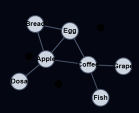
Depth First Search Traversal
Depth First Search is said to go “deep” because it visits a vertex, then an adjacent vertex, and then that vertex’ adjacent vertex, and so on, and in this way the distance from the starting vertex increases for each recursive iteration.
Example
class Graph:
def init(self, size):
self.adj_matrix = [[0] * size for _ in range(size)]
self.size = size
self.vertex_fooddata = [”] * size
def add_edge(self, u, v):
if 0 <= u < self.size and 0 <= v < self.size:
self.adj_matrix[u][v] = 1
self.adj_matrix[v][u] = 1
def add_vertex_fooddata(self, vertex, data):
if 0 <= vertex < self.size:
self.vertex_fooddata[vertex] = data
def print_graph(self):
print(“Adjacency Matrix:”)
for row in self.adj_matrix:
print(‘ ‘.join(map(str, row)))
print(“\nVertex Food Data:”)
for vertex, data in enumerate(self.vertex_fooddata):
print(f”Vertex {vertex}: {data}”)
def dfs_util(self, v, visited):
visited[v] = True
print(self.vertex_fooddata[v], end=’ ‘)
for i in range(self.size):
if self.adj_matrix[v][i] == 1 and not visited[i]:
self.dfs_util(i, visited)
def dfs(self, start_vertex_fooddata):
visited = [False] * self.size
start_vertex = self.vertex_fooddata.index(start_vertex_fooddata)
self.dfs_util(start_vertex, visited)
g = Graph(7)
g.add_vertex_fooddata(0, ‘Apple’)
g.add_vertex_fooddata(1, ‘Bread’)
g.add_vertex_fooddata(2, ‘Coffee’)
g.add_vertex_fooddata(3, ‘Dosa’)
g.add_vertex_fooddata(4, ‘Egg’)
g.add_vertex_fooddata(5, ‘Fish’)
g.add_vertex_fooddata(6, ‘Grape’)
g.add_edge(3, 0) # Dosa – Apple
g.add_edge(0, 2) # Apple – Coffee
g.add_edge(0, 3) # Apple – Dosa
g.add_edge(0, 4) # Apple – Egg
g.add_edge(4, 2) # Egg – Coffee
g.add_edge(2, 5) # Coffee – Fish
g.add_edge(2, 1) # Coffee – Bread
g.add_edge(2, 6) # Coffee – Grape
g.add_edge(1, 5) # Bread – Fish
g.print_graph()
print(“\nDepth First Search starting from vertex Dosa:”)
g.dfs(‘Dosa’)
Output:
Adjacency Matrix:
0 0 1 1 1 0 0
0 0 1 0 0 1 0
1 1 0 0 1 1 1
1 0 0 0 0 0 0
1 0 1 0 0 0 0
0 1 1 0 0 0 0
0 0 1 0 0 0 0
Vertex Food Data:
Vertex 0: Apple
Vertex 1: Bread
Vertex 2: Coffee
Vertex 3: Dosa
Vertex 4: Egg
Vertex 5: Fish
Vertex 6: Grape
Depth First Search starting from vertex Dosa:
Dosa Apple Coffee Bread Fish Egg Grape
The DFS traversal starts when the dfs() method is called.
The visited array is first set to false for all vertices, because no vertices are visited yet at this point.
The visited array is sent as an argument to the dfs_util() method. When the visited array is sent as an argument like this, it is actually just a reference to the visited array that is sent to the dfs_util() method, and not the actual array with the values inside. So there is always just one visited array in our program, and the dfs_util() method can make changes to it as nodes are visited .
For the current vertex v, all adjacent nodes are called recursively if they are not already visited.
dfs() முறை அழைக்கப்படும்போது DFS பயணம் தொடங்குகிறது.
இந்தக் கட்டத்தில் எந்த முனைகளும் இன்னும் பார்வையிடப்படாததால், முதலில் அனைத்து முனைகளுக்கும் ‘visited’ அணிவரிசை ‘false’ என அமைக்கப்படுகிறது.
‘visited’ அணிவரிசை dfs_util() முறைக்கு ஒரு வாதமாக அனுப்பப்படுகிறது. ‘visited’ அணிவரிசை இந்த வழியில் ஒரு வாதமாக அனுப்பப்படும்போது, அது உண்மையில் மதிப்புகளைக் கொண்ட உண்மையான அணிவரிசை அல்ல, மாறாக ‘visited’ அணிவரிசைக்கான ஒரு குறிப்பு மட்டுமே dfs_util() முறைக்கு அனுப்பப்படுகிறது. எனவே, நமது நிரலில் எப்போதும் ஒரே ஒரு ‘visited’ அணிவரிசை மட்டுமே இருக்கும், மேலும் முனைகள் பார்வையிடப்படும்போது dfs_util() முறையானது அதில் மாற்றங்களைச் செய்ய முடியும்.
தற்போதைய முனை v-க்கு, அருகிலுள்ள அனைத்து முனைகளும் ஏற்கனவே பார்வையிடப்படவில்லை என்றால், அவை மீள்சுழல் முறையில் அழைக்கப்படுகின்றன.
Breadth First Search Traversal
Breadth First Search visits all adjacent vertices of a vertex before visiting neighboring vertices to the adjacent vertices. This means that vertices with the same distance from the starting vertex are visited before vertices further away from the starting vertex are visited.
அகல முதல் தேடல் வழிமுறை
அகல முதல் தேடல் முறையில், ஒரு முனையின் அருகிலுள்ள முனைகளுக்குச் செல்லும் முன், அந்த முனையின் அனைத்து அண்டை முனைகளும் பார்வையிடப்படுகின்றன. இதன் பொருள், தொடக்க முனையிலிருந்து ஒரே தூரத்தில் உள்ள முனைகள், தொடக்க முனையிலிருந்து அதிக தூரத்தில் உள்ள முனைகளுக்குச் செல்வதற்கு முன்பு பார்வையிடப்படுகின்றன என்பதாகும்.
Example:
class Graph:
def init(self, size):
self.adj_matrix = [[0] * size for _ in range(size)]
self.size = size
self.vertex_fooddata = [”] * size
def add_edge(self, u, v):
if 0 <= u < self.size and 0 <= v < self.size:
self.adj_matrix[u][v] = 1
self.adj_matrix[v][u] = 1
def add_vertex_fooddata(self, vertex, data):
if 0 <= vertex < self.size:
self.vertex_fooddata[vertex] = data
def print_graph(self):
print(“Adjacency Matrix:”)
for row in self.adj_matrix:
print(‘ ‘.join(map(str, row)))
print(“\nVertex Data:”)
for vertex, data in enumerate(self.vertex_fooddata):
print(f”Vertex {vertex}: {data}”)
def bfs(self, start_vertex_fooddata):
queue = [self.vertex_fooddata.index(start_vertex_fooddata)]
visited = [False] * self.size
visited[queue[0]] = True
while queue:
current_vertex = queue.pop(0)
print(self.vertex_fooddata[current_vertex], end=’ ‘)
for i in range(self.size):
if self.adj_matrix[current_vertex][i] == 1 and not visited[i]:
queue.append(i)
visited[i] = True
g = Graph(7)
g.add_vertex_fooddata(0, ‘Apple’)
g.add_vertex_fooddata(1, ‘Bread’)
g.add_vertex_fooddata(2, ‘Coffee’)
g.add_vertex_fooddata(3, ‘Dosa’)
g.add_vertex_fooddata(4, ‘Egg’)
g.add_vertex_fooddata(5, ‘Fish’)
g.add_vertex_fooddata(6, ‘Grape’)
g.add_edge(3, 0) # Dosa – Apple
g.add_edge(0, 2) # Apple – Coffee
g.add_edge(0, 3) # Apple – Dosa
g.add_edge(0, 4) # Apple – Egg
g.add_edge(4, 2) # Egg – Coffee
g.add_edge(2, 5) # Coffee – Fish
g.add_edge(2, 1) # Coffee – Bread
g.add_edge(2, 6) # Coffee – Grape
g.add_edge(1, 5) # Bread – Fish
g.print_graph()
print(“\nBreadth First Search starting from vertex Dosa:”)
g.bfs(‘Dosa’)
Output:
Adjacency Matrix:
0 0 1 1 1 0 0
0 0 1 0 0 1 0
1 1 0 0 1 1 1
1 0 0 0 0 0 0
1 0 1 0 0 0 0
0 1 1 0 0 0 0
0 0 1 0 0 0 0
Vertex Data:
Vertex 0: Apple
Vertex 1: Bread
Vertex 2: Coffee
Vertex 3: Dosa
Vertex 4: Egg
Vertex 5: Fish
Vertex 6: Grape
Breadth First Search starting from vertex Dosa:
Dosa Apple Coffee Egg Bread Fish Grape
The bfs() method starts by creating a queue with the start vertex inside, creating a visited array, and setting the start vertex as visited.
The BFS traversal works by taking a vertex from the queue, printing it, and adding adjacent vertices to the queue if they are not visited yet, and then continue to take vertices from the queue in this way. The traversal finishes when the last element in the queue has no unvisited adjacent vertices.
bfs() முறைமையானது, தொடக்க முனையைக் கொண்ட ஒரு வரிசையை உருவாக்குவதன் மூலமும், ஒரு பார்வையிடப்பட்ட அணிவரிசையை உருவாக்குவதன் மூலமும், தொடக்க முனையைப் பார்வையிடப்பட்டதாகக் குறிப்பதன் மூலமும் தொடங்குகிறது.
BFS கடந்துசெல்லும் செயல்முறையானது, வரிசையிலிருந்து ஒரு முனையை எடுத்து, அதைப் பதிப்பித்து, இதுவரை பார்வையிடப்படாத அருகிலுள்ள முனைகளை வரிசையில் சேர்ப்பதன் மூலமும், பின்னர் இந்த வழியில் வரிசையிலிருந்து முனைகளைத் தொடர்ந்து எடுப்பதன் மூலமும் செயல்படுகிறது. வரிசையில் உள்ள கடைசி உறுப்புக்கு பார்வையிடப்படாத அருகிலுள்ள முனைகள் எதுவும் இல்லாதபோது இந்த கடந்துசெல்லும் செயல்முறை முடிவடைகிறது.